Refererences:
R. Ramakrishnan and J. Gehrke, Database Management Systems, 4.2-4.3
1. Relations
1.1. Definitions
Definition of Domain: domain is a set of values with the same data type.
Definition of Cartesian Product: For given domains $D_1, D_2, ..., D_n$, their Cartesian product is defined as
这里的笛卡尔积严格地讲是广义笛卡尔积(Extended Cartesian Product). 在不会出现混淆的情况下广义笛卡尔积也称为笛卡尔积.
更加精确的定义: 两个分别为 $n$ 目和 $m$ 目的关系 $R$ 和 $S$ 的广义笛卡尔积是一个 $(n+m)$ 列的元组的集合. 元组的前 $n$ 列是关系 $R$ 的一个元组, 后 $m$ 列是关系 $S$ 的一个元组. 若 $R$ 有 $k_1$ 个元组, $S$ 有 $k_2$ 个元组, 则关系 $R$ 和关系 $S$ 的广义笛卡尔积有 $k_1×k_2$ 个元组. 记作:
Definition of Tuple: Every element of a cartesian product $(d_1, d_2, …, d_n)$ is called a $n$-tuple or just a tuple.
Definition of Component (分量): every (column) value of a $n$-tuple $(d_1, d_2,\dots, d_n)$ i.e. $d_i$ is called a component of the tuple.
Definition of Cardinal number (基数): If every $D_i\ (i=1, 2,\ldots, n)$ is a finite set, then the cardinal number of $D_1\times D_2\times\ldots\times D_n$ is recursively defined as
Definition of Relation: Every element of the set $D_1\times D_2\times\ldots\times D_n$ is called a relation on the domains $D_1, D_2, ..., D_n$, denoted by $R(D_1, D_2, ..., D_n)$, where:
- $R: $ is the name of the relation
- $n:$ is called the degree (目/度) of the relation
Definition of Attribute: Note that every column can correspond to the same domain, so to distinguish them, each column must be given a name, called an attribute. A relation of $n$ degrees must have $n$ attributes.
Definition of Key
- Candidate Key: A set of attributes that just uniquely identifies a tuple (by just I mean the smallest set of attributes that can uniquely identify a tuple)
- Super Key: A set of attributes that uniquely identifies a tuple.
- Primary Key: Any one of the candidate keys can be a primary key.
- Prime Attribute: All attributes in a candidate key are called prime attributes
- Non-Prime/Non-key Attribute: All attributes that are not in the candidate key are called non-prime attributes
All attributes in a relation are either prime or non-prime.
1.2. Relations
在数据库中, 关系可以分成如下几类
- 基本关系 (基本表或基表): 实际存在的表, 是实际存储数据的逻辑表示.
- 查询表: 查询结果对应的表.
- 视图表: 由基本表或其他视图表导出的表, 是虚表, 不对应实际存储的数据.
我们在这里主要研究基本关系, 基本关系具有如下的性质.
- 列是同质的 (Homogeneous): 每一列中的分量是同一类型的数据, 来自同一个域
- 不同的列可出自同一个域: 其中的每一列称为一个属性, 不同的属性要给予不同的属性名
- 列的顺序无所谓: 列的次序可以任意交换
- 任意两个元组的候选键不能相同
- 行的顺序无所谓: 行的次序可以任意交换
- 分量必须取原子值
1.3. Relational Schema
Definition: formally, $\text{relational schema}$ can be defined as $R(U, D, DOM, F)$, where
- $R:$ 关系名
- $U:$ 组成该关系的属性的集合
- $D:$ $U$ 中属性所来自的域
- $DOM:$ 属性向域的映象集合 (常常直接说明为属性的类型 & 长度)
- $F:$ 属性间数据的依赖关系的集合
也可以简记为 $R(U)$ 或 $R(A_1, A_2, ..., A_n)$, where $A_1, A_2, ..., A_n$ 为属性名称
Normally, we can consider relation as an instance of a given relational schema. But intuitionally I don’t see any differences
1.4. Relational Database
在一个给定的应用领域中, 所有关系的集合构成一个关系数据库
Definition of Type and Value of a relational schema
- Type: 关系数据库模式, 是对关系数据库的描述
- Value: 关系模式在某一时刻对应的关系的集合, 通常称为关系数据库
2. Relational Integrity
2.1. Constraints
- Entity Integrity Constraint: 关系数据库中, 主键/主属性不能为
NULL(基本表通常对应现实世界的一个实体集, 而现实世界中的实体是可区分的, 即它们具有某种唯一性标识. ) - Referential Integrity Constraint: 关系数据库中, 确保在一个表中引用另一个表时, 引用有效的行. i.e. 外键值必须在关联表中存在. (在关系模型中实体及实体间的联系都是用关系来描述的, 自然存在着关系与关系间的引用)
- User-Defined Integrity Constraint: 由用户定义的一组规则, 用于限制对表的访问和维护, 例如 CHECK 约束, 触发器等.
其中, 前两者由关系系统自动支持, 后者应用时需要遵循的语义规则, 体现了具体领域中的语义约束
Definition of Foreign Key
说白了就是在当前表中不是主键但是在别的表中是主键的键
设 $F$ 是基本关系 $R$ 的一个或一组属性, 但不是关系 $R$ 的键 (key). 如果 $F$ 与基本关系 $S$ 的主键 $K_s$ 相对应, 则称 $F$ 是 $R$ 的外键. where
- $R:$ 参照 / 引用关系 (Referencing Relation)
- $S:$ 被参照 / 被引用关系 (Referenced Relation) / 目标关系 (Target Relation)
Definition of Referential Integrity Constraint
若属性 (或属性组) $F$ 是基本关系 $R$ 的外键它与基本关系 $S$ 的主键 $K_s$ 相对应 (基本关系 $R$ 和 $S$ 不 一定是不同的关系), 则对于 $R$ 中每个元组在 $F$ 上的值必须为下列两种情况之一
- 空值 ($F$ 的每个属性值均为空值)
- $S$ 中某个元组的主键值
3. Relational Algebra
关系代数是一种抽象的查询语言, 它用对关系的运算来表达查询.
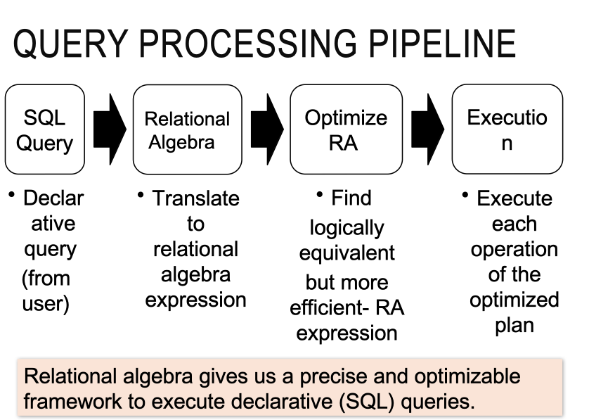
Observe that queries in algebra are composed using a collection of operators. A fundamental property is that every operator in the algebra accepts (one or two) relation instances as arguments and returns a relation instance as the result.
Codd (the C of BCNF) 是关系代数(数据库)的创始人, 他提出了六种原始运算 (还有其他的运算可以由原始运算导出)
选择, 投影, Descartes积, 并集, 差集, 重命名. 其中,
- 并集, 差集和Descartes积是集合操作中的基本运算
- 选择, 投影和重命名是关系操作中的基本运算.
除此之外, 关系代数(数据库)中还有一些别的运算, 包括连接和类似连接的计算, 还有除法
3.1. Set Operations

Definition of Union
If two relations $R$ and $S$ have the same schema (so their each attribute should come from the same domain respectively).
Then the union of these two relations is
Definition of Difference
If two relations $R$ and $S$ have the same schema. Then the difference between $R$ and $S$ is
也就是在数据库中, 具有相同性质和数量列的两个表, 行可以相减 (集合意义上的减)
Definition of Intersection
If two relations $R$ and $S$ have the same schema. Then the intersection of these two relations is
The reason we use such a definition instead of the native one is because this operation is not raw in the relational algebra, i.e. we can derive it from the difference operation.
3.2. Related Symbols
-
$R:$ 关系模式 (对应于关系数据库中的一张表)
-
$t\in R:$ $t$ 是 $R$ 的一个元组 (这里可见, 我们认为表的基本元素是行而不是列)
-
$t[A_i]:$ 元组 $t$ 中相应于属性 $A_i$ 的一个分量
-
$A = \{A_{i_1}, A_{i_2}, ..., A_{i_k}\}:$ $A$ 称为属性列或属性组.
-
$t[A]:$ 元组 $t$ 中相应于属性组 $A$ 中所有属性的分量集合
-
$\bar A:$ $\{A_{1}, A_{2}, ..., A_{n}\} - A$
3.3. Relational Operations
1. Selection:
Given a relation (table) $R$ and a condition $\varphi$, return some tuples of this relation
Definition of Selection: 广义选择 是写为 $\sigma _{\varphi }(R)$ 的一元运算, 这里的 $\varphi$ 是由正常选择中所允许的原子和逻辑算子 $\land , \lor, \lnot$ 构成的命题公式. 这种选择选出 $R$ 中使 $\varphi$ 成立的所有元组. 可以表示为:
where $\varphi:$ 选择条件, 是一个逻辑表达式, 取值为“真”或“假”
2. Projection:
Given a relation (table) $R$ and a set of Attributes $A_1, A_2, \ldots, A_n$
Definition of Projection: 投影是写为 $\Pi_{A_1,\ldots,A_n}(R)$ 的一元运算, 这里的 $A_{1},...,A_{n}$ 是属性名字的集合. 这种投影的结果定义为当所有在 $R$ 中的元组被限制为集合 $\{A_{1},...,A_{n}\}$ 的时候所获得的集合. 可以表示为:
其中, $A$ 为 $R$ 中的一些属性列的集合
3. Cartesian Product:
Given two relations $R(A_1, A_2, \ldots, A_n)$ and $S(B_1,B_2,\ldots,B_m)$ with no common attributes (even if they have, we still treat these two attributes as different), return a new relation with $m+n$ attributes
where $t_r \textsf{ concat } t_s$ is the concatenation of two tuples $t_r$ and $t_s$.
4. Rename:
Given a relation $R(A_1, A_2, \ldots, A_n)$, rename the attributes to $B_1, B_2, \ldots, B_n$
where $B_1, B_2, \ldots, B_n$ are the new names of the attributes.
5. Join:
5.1. $\theta$-Join: Inner Join:
Given two relations $R$ and $S$ and a condition $\theta$, return a new relation with the same schema as the Cartesian product of these two relations, but only the tuples that satisfy the condition are kept.
连接运算就是从两个关系的笛卡尔积中选取属性之间满足一定条件的元组进行连接, i.e.
or not so formally:
where
- $A$ 和 $B:$ 分别为 $R$ 和 $S$ 上度数相等且可比的属性组
- $\theta:$ 比较运算符
比较特殊地, Join 包括但不限于有 Equijoin (where $\theta$ is $\text{equivalent}$) 的情况. 更加特殊地, Equijoin 包括但不限于有 Natural join (where lines / tuples are $\text{unique}$) 这一情况.
一般来说, $\Join$ 符号就表示自然连接.
2. Natural Join: Inner Join:
Natural Join is different from $\theta$-Join in that it regards two same attributes in two relations as the same attribute, and only keeps one of them in the result.
3. Outer Join:
悬挂元组 (Dangling tuple): 两个关系 $R$ 和 $S$ 在做自然连接时, 关系 $R$ 中某些元组有可能在 $S$ 中不存在公共属性上值相等的元组, 从而造成 $R$ 中这些元组在操作时被舍弃了. 这些被舍弃的元组称为悬浮元组.
如果把悬浮元组也保存在结果关系中, 而在其他属性上填空值 (Null), 就叫做外连接
- 左外连接 (left join / left outer join): 只保留左边关系 $R$ 中的悬浮元组
- 右外连接 (right join / right outer join): 只保留右边关系 $S$ 中的悬浮元组
6. Division:
Given two relations $R (X, Y)$ and $S(Y, Z)$
$R$ 中的 $Y$ 与 $S$ 中的 $Y$ 可以有不同的属性名, 但必须出自相同的域集. $R$ 与 $S$ 的除运算得到一个新的关系 $P(X)$, $P$ 是 $R$ 中满足下列条件的元组在 $X$ 属性列上的投影:
元组在 $X$ 上分量值 $x$ 的象集 $Y_x$ 包含 $S$ 在 $Y$ 上投影的集合, 记作:
where
- $Y_x:$ $x$ 在 $R$ 中的象集 ( $R$ 中属性组 $X$ 上值为 $x$ 的诸元素在 $Y$ 分量上的集合)
- $x = t_r [X]$