We have alternative ways of evaluating a given query
- Equivalent Expressions
- Different Algorithms for Each Operation
1. Query Performance
Consider such a query:
1 | SELECT i.name, C.title |
An Evaluation Plan defines exactly what algorithm is used for each operation, and how the execution of the operations is coordinated. For example we can parse the query into such a query tree:
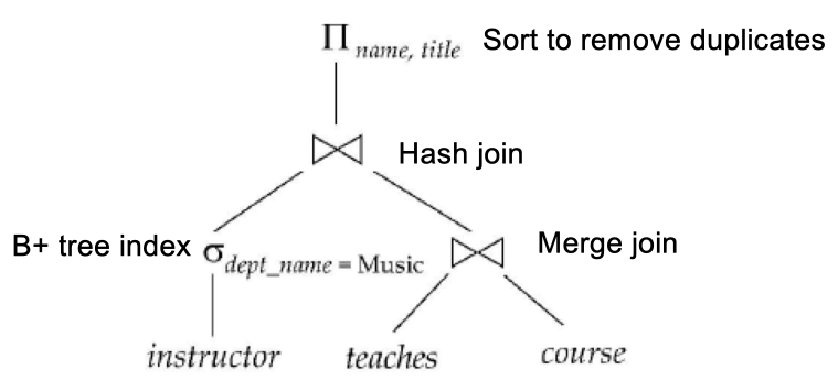
Cost difference between evaluation plans for a query can be enormous (e.g. seconds vs. days in some cases)
Cost-based query optimization includes the following steps:
- Generate logically equivalent expressions using equivalence rules.
- Annotate resultant expressions to get alternative query plans.
- Choose the cheapest plan based on estimated cost.
Estimation of plan cost based on:
- Statistical information about relations. Examples: number of tuples, number of distinct values for an attribute.
- Statistics estimation for intermediate results to compute cost of complex expressions.
- Cost formulae for algorithms, computed using statistics.
Some Equivalence Rules:
- Conjunctive selection operations can be deconstructed into a sequence of individual selections.
$$\sigma_{\theta_1 \wedge \theta_2}(R) = \sigma_{\theta_1}(\sigma_{\theta_2}(R))
$$
- Selection operations are commutative.
$$\sigma_{\theta_1 \wedge \theta_2}(R) = \sigma_{\theta_2 \wedge \theta_1}(R)
$$
- Only the last in a sequence of projection operations is needed, the others can be omitted.
$$\pi_{A_1}(\pi_{A_2}(R)) = \pi_{A_1}(R)
$$
- Selections can be combined with Cartesian products and theta joins.
$$\begin{aligned}
\sigma_{\theta_1}(R \times S) &= R\Join_{\theta_1}S \\
\sigma_{\theta_1}(R \Join_{\theta_2} S) &= R \Join_{\theta_2 \wedge \theta_1} S
\end{aligned}
$$
- Theta-join operations (and natural joins) are commutative.
$$R \Join_{\theta} S = S \Join_{\theta} R
$$
- Natural join operations are associative:
$$R \Join S \Join T = R \Join (S \Join T)
$$
- Theta-join operations are equivalent in the following manner:
$$(R \Join_{\theta_1} S) \Join_{\theta_2} T = R \Join_{\theta_1 \wedge \theta_2} (S \Join T)
$$
-
The selection operation distributes over the theta join operation under the following two conditions:
- When all the attributes in $\theta_0$ involve only the attributes of R being joined.
$$\sigma_{\theta_0}(R \Join_{\theta} S) = \sigma_{\theta_0}(R) \Join_{\theta} S $$- When $θ_1$ involves only the attributes of R and $θ_2$ involves only the attributes of S.
$$\sigma_{\theta_1}(R) \Join_{\theta} \sigma_{\theta_2}(S) = \sigma_{\theta_1 \wedge \theta_2}(R \Join S) $$ -
The projection operation distributes over the theta join operation as follows:
- If $\theta$ involves only the attributes from $L_1\cup L_2$
$$\pi_{L_1\cup L_2}(R \Join_{\theta} S) = \pi_{L_1}(R) \Join_{\theta} \pi_{L_2}(S) $$