1. Feature Selection and Dimensionality Reduction
1.1. Feature Selection
关于特征工程, 可以查看我的这篇笔记
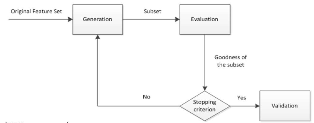
特征选择本质上是搜索问题. 也就是说, 对于 $n$ 个原始特征构成的大小为 $2^n-1$ 的特征空间, 如何搜索最优的特征子集
- 前向搜索: 起点为空集
- 后向搜索: 起点为全集
- 双向搜索
很自然地, 我们需要一些特征评估函数来判断我们抽选出的特征是否合适. 特征评估函数大体可以分成三类:
- 过滤式: 使用评价准则来增强特征与类的相关性, 削减特征之间的相关性. 具体来说, 包括距离度量(方差法), 信息度量(互信息熵), 依赖性度量( $\text{Pearson}$ 相关系数, $\chi^2$检验) 以及一致性度量.
- 封装式: 特征及其与任务目标(分类, 回归, 聚类等)的相关性. 具体来说, 可以设计分类错误率来度量
- 嵌入式: 模型正则化
,
1.2. Dimensionality Reduction
数据降维有很多好处, 包括但不限于:
- 降低over-fitting风险
- 增加解释性
- 去除冗余特征
2. LDA
详情查看我的这篇数据科学笔记
3. PCA
详情查看我的这篇数据科学笔记
4. ICA
4.1. FA
Factor Analysis (因素分析, FA) 假设数据是由多个物理源所产生(并附加测量噪声), 因素分析将数据解释为少数不相关因素的累加.
to be continued
5. LLE
详情查看我的这篇数据科学笔记
6. ISOMAP
6.1. MDS
1. Principles
Multi-Dimensional Scaling (多维缩放, MDS) 和PCA算法一样尝试寻找整个数据空间的一个线性近似, 从而把数据嵌入到低维空间中
- MDS算法在嵌入时尝试保留所有数据点对之间的距离(假设这些距离已经测出)
- 如果空间是欧式空间的话, 这两种方法等价
已知高维上样本点两两之间的距离, 尝试在低维上 (通常是2维, 但是可以是任意维) 找到一组新的样本点, 使降维后两点间的距离与它们在高维上的距离相等
假设原始数据集 $\boldsymbol x_1,\boldsymbol x_2, \ldots\boldsymbol x_N\in \mathbb R^M$, 降维后的目标数据集为 $\boldsymbol z_1, \boldsymbol z_2, \ldots, \boldsymbol z_N\in \mathbb R^L$ (其中 $L<M$). 很自然地, 我们定义了一些**基于距离的**目标函数, 来刻画当前映射的优劣. 有两种常见的目标函数
(1) Kruskal-shephard scaling (最小二乘法)
(2) Sammon mapping
对误差加权, 产生非线性
但仍可以优化. 我们可以定义**基于相似度的**MDS. 我们假设: 数据点间的相似度可以替代距离. 预处理: 数据去中心化 (数据科学常见的手段). 那么两个点 $\boldsymbol x_i,\boldsymbol x_j$ 的相似度 $s_{ij}$ 定义为
此时我们的目标是最小化如下的目标函数
2. Classic Linear MDS
经典线性 MDS 的思路如下:
- 去中心化原始空间数据 $\boldsymbol x_1,\boldsymbol x_2,\ldots,\boldsymbol x_n$, 计算点对距离 $D$ ($D_{ij}=\|\boldsymbol x_i-\boldsymbol x_j\|$, 去中心化指的是 $\boldsymbol x_i\leftarrow \boldsymbol x_i-\boldsymbol {\bar x}$ )
- 求投影后空间数据点内积矩阵 $B=\boldsymbol z\boldsymbol z^{\mathsf T}$
- 根据 $B$, 求解投影后数据 $\boldsymbol z_1, \boldsymbol z_2, \ldots, \boldsymbol z_n$
- 得出投影矩阵
我们发现去中心化有这样良好的性质
此时, 令 $\operatorname{dist}_{ij}=\|\boldsymbol z_i-\boldsymbol z_j\|$, 有:
则令 $B=\boldsymbol z\boldsymbol z^{\mathsf T}$:
这里用一点基本的和式变换, 可以得到
形式化地, 我们令
那么有
3. Steps
- 计算由高维上每对点相似度组成的矩阵 $D$, $D_{ij}=\|\boldsymbol x_i-\boldsymbol x_j\|$
- 计算 $J=\displaystyle (1-\frac 1 n)\cdot I_n$ (这儿 $I_n$ 是 $n\times n$ 单位矩阵, $n$ 是数据点个数)
- 计算 $B=\displaystyle -\frac 1 2JDJ^{\mathsf T}$
- 找到 $B$ 的 $L$ 个最大特征值 $\lambda_i$, 和相对应特征向量 $\xi_i$
- 用特征值组成对角矩阵 $V$ 并且用特征向量作成矩阵 $P$ 的列向量
- 计算嵌入= $PV^{\frac 1 2 }$
6.2. ISOMAP
流形空间: 任何现实世界中的对象均可以看做是低维流形在高维空间的嵌入(嵌入可以理解为表达)
如: 圆在直角坐标系是二维的, 但在极坐标系是一维的
Isometric Feature Mapping (等距特征映射, ISOMAP) 通过检查所有点对间的距离和计算全局测地线的方法来最小化全局误差.
The classical MDS algorithm works fine on flat manifolds (dataspaces). However, we are interested in manifolds (流形) that are not flat, and this is where Isomap comes in. The algorithm has to construct the distance matrix for all pairs of datapoints on the manifold, but there is no information about the manifold, and so the distances can’t be computed exactly.
ISOMAP approximates them by assuming that the distances between pairs of points that are close together are good, since over a small distance the non-linearity of the manifold won’t matter. It builds up the distances between points that are far away by finding paths that run through points that are close together, i.e., that are neighbours, and then uses normal MDS on this distance matrix.
具体来说, ISOMAP算法包括如下的四个步骤:
- Construct the pairwise distances between all pairs of points
- Identify the neighbours of each point to make a weighted graph $G$
- Estimate the geodesic distances $d_G$ by finding shortest paths
- Apply classical MDS to the set of $d_G$