Definition of Markov chain

$$\huge\textbf{Definition of Markov chain} $$

1. Stochastic Matrices

$\textbf{Definition 4.1.}\quad$ Let $I$ be a countable set.

(1) A square matrix $P = ((p_{ij} ))_{i,j∈I}$ is called a $\textbf{stochastic matrix}$ if

$$ \begin{align} i.&: \forall i,j\in I: p_{ij}>0\\ ii.&: \forall i \in I: \sum_{j\in I}p_{ij}=1 \end{align} $$

(2) A square matrix $P$ is called a $\textbf{sub-stochastic matrix}$ if it satisfies $i.$ and $iii$

$$ iii.: \forall i \in I: \sum_{j\in I}p_{ij}\leqslant 1 $$

(3) A square matrix $P$ is called a $\textbf{doubly-stochastic matrix}$ if $P$ and $P^{\textsf T}$ are both stochastic matrices.

The way to think of the entry $p_{ij}$ is, roughly, “the probability of going to state $j$ next, given that we are at state $i$ now”. We will make this more precise, but for now think of these probabilities as “transition probabilities”. As such, a stochastic matrix is also commonly called a transition/Markov matrix, or a generator.

$\textbf{Definition 4.2.}\quad$ A $\textbf{directed graph}$ $G = (V, E)$ is a set of vertices $V$ and collection of directed edges $(i, j) ∈ E ⊂ V × V$ from vertex $i$ to vertex $j$. A $\textbf{weighed graph}$ $(V, E, W)$ is a graph $(V, E)$ with the weight of an edge $e = (i, j)$ given by $w_e = w_{ij}$ . We will assume that $w_{ij} = 0$ $\text{iff}$ $(i, j)$ is not an edge in the graph.

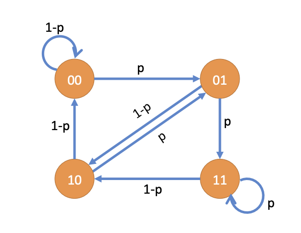
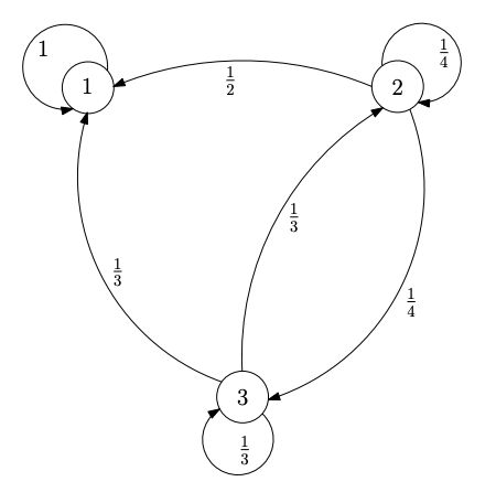
Given a Stochastic matrix $P = ((p_{ij} ))_{i,j∈I}$ we can define a weighed directed graph with vertex set I and edge weight of $(i, j)$ given by $p_{ij}$ . Note that, $\sum_{j∈I} p_{ij} = 1$ for all $i$ implies that the total weight of all the out-edges from the vertex $i$ is 1. The picture below shows the weighted direct graph of a the stochastic matrix

$$P=\left[\begin{array}{ccc}1 & 0 & 0 \\ 1 / 2 & 1 / 4 & 1 / 4 \\ 1 / 3 & 1 / 3 & 1 / 3\end{array}\right] $$

$\textbf{Definition 4.4.}\quad$

(1) A path in a directed graph $G = (V, E)$ is a collection of edges $(i_0, i_1), (i_1, i_2),\dots,(i_{n−1}, i_n)$ where $i_0, i_1,\ldots , i_n \in V$ . Moreover, the length of a path is the number of edges in this path, and the weight of a path is defined as

$$ \prod_{\text{edges in the path}} \text{edge weights}. $$

(2) A cycle is a path with the same starting and ending vertices.

$\textbf{Theorem 4.7.}$ For a stochastic matrix $P$, the following statements hold:

(i) $\operatorname{spec}(P) ⊆ B(0, 1)$

(ii) $\forall i:p_{ii} > 0\implies \operatorname{spec}(P) ⊆ B(0, 1) ∪ \{1\}$.

$Proof.$

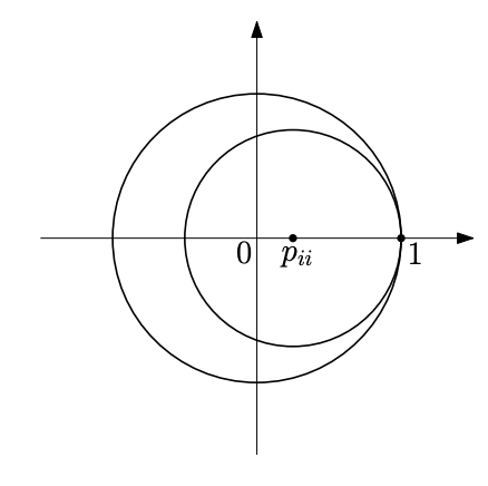
i. $\forall i:R_i = \displaystyle \sum_{j\not =i} |p_{ij} | = 1 − p_{ii}$. Suppose $z$ is an eigenvalue of $P$. Then by $\textbf{Gershgorin circle theorem}$, $z ∈ B(p_{ii}, 1 − p{ii})$ and thus, $|z| ⩽ 1$.

ii. Follows from the fact that $B(p_{ii}, 1 − p_{ii}) ⊆ \overline{B(0, 1)} ∪ \{1\}$ if $p_{ii} > 0$. (as the folowing picture)

2. Discrete Time Markov Chains

2.1. Definitions

$\textbf{Definition 4.8.}\quad$ Given a probability space $(\Omega, \mathcal F, \mathbb P)$, a set $I$, and an ordered set $\mathcal T$ , a stochastic process (with values in $I$) is a collection of random variables $(X_t)_{t∈\mathcal T}$ such that $X_t: \Omega \to I$ is a random variable for each $t \in\mathcal T$ . We call $I$ the state space of the stochastic process and $\mathcal T$ the time domain. Moreover, if $\mathcal T$ is countable ( $e.g.$, $\mathbb N = {0, 1, 2, . . .}$), then we get a $\textbf{discrete-time stochastic process}$.

A stochastic process is a function of two variables, and could be written $X(ω, t)$. But it is more commonly written as $X_t(ω)$, since we think of these two variables differently. For each fixed $t ∈\mathcal T$, $X_t$ is a random variable, and once we choose a specific outcome in $Ω$, we have the number $X_t(ω)$. In this sense, a stochastic process is a sequence of random variables, indexed by time. On the other hand, for each fixed $ω ∈ Ω$, $X_t(ω)$ is a curve or path in the set $I$. So that we can think of a stochastic process as a random variable whose values are paths in $I$. Both of these points of view are valid and each will be useful in various contexts.

$\textbf{Definition 4.9.}\quad$ Consider a discrete-time stochastic process $(X_t)_{t⩾0}$ defined on an underlying probability space $(\Omega, \mathcal F, \mathbb P)$ and taking values in the set $I$. The random process is called a $\textbf{discrete-time Markov chain}$ with initial distribution $\lambda$ and transition matrix $P$ if,

(1) $X_0\sim\lambda$, where $\lambda$ is the initial distribution

(2) $\mathbb P(X_n=j\mid X_0=x_0, X_1=x_1, \ldots,X_{n-1}=i=\mathbb P(X_n = j|X_{n−1} = i) = p_{ij})$, which implies, given $X_{n−1}$, the random number $X_n$ is independent of the history, $X_0, X_1, \ldots , X_{n−2}$.

Here, $P = ((p_{ij}))$ is called the transition matrix and we will use the notation

$$ (X_t)_{t⩾0} \sim \operatorname{Markov}(\lambda, P) $$

If $p_{ij}$ s are independent of time (consequently, transition matrix $P$ is also independent of time), then the Markov chain is called the $\textbf{time-homogeneous}$ Markov chain.

2.2. Examples

$\textbf{Random Walk on integers}$: Consider the set of integers and a Markov chain $(X_i)_{i⩾0}$. The random variables take integer values, $i.e.$ $I = \mathbb Z$. Consider $X_0 = 1$ (or some other distribution $\lambda$). The value of the random variable in the next step increases by 1 with probability 1/4, decreases by 1 with probability 1/4, and stays the same with probability 1/2. This can be formally written as

$$p_{i j}=\left\{\begin{array}{l}1 / 4, \quad j=i+1 \\ 1 / 4, \quad j=i-1 \\ 1 / 2, \quad j=i \\ 0, \quad \text { otherwise }\end{array}\right. $$

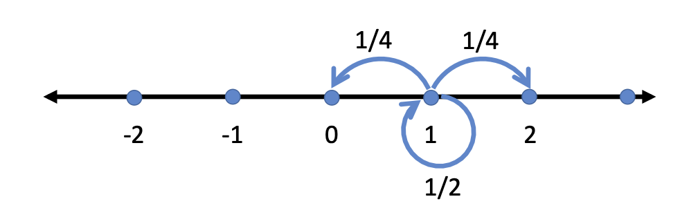
The transition probability matrix, $P$, has a special structure (tridiagonal matrix, 三对角矩阵) in this example
and we write, $(X_t)_{t⩾0} \sim \text{Markov}(\lambda, P)$. This process denoted as $(X_t)_{t⩾0} \sim \text{Markov}(\lambda, P)$, is also called $\textbf{Lazy Random Walk}$. It is called lazy since the Markov chain stays the same with a probability of 1/2.

$\textbf{Random Walk with absorption:}$ Consider an integer $n$ and a Markov chain $(X_t)_{t⩾0}$. The random variables take integer values in $I = \{−N, −(N − 1), \ldots , −1, 0, 1, . . . , N\}$. Consider $X_0 = 1$ (or some distribution $\lambda$). The value of the random variable in the next step increases by 1 with probability 1/4, decreases by 1 with probability 1/4, and stays the same with probability 1/2. Moreover, once the random variable reaches the end, $\{±N\}$, the random variable stays there with a probability of 1. We can write the transition probability matrix as,

$$P=\left[\begin{array}{cccccc}1 & 0 & 0 & 0 & \ldots & 0 \\ 0.25 & 0.5 & 0.25 & 0 & \ldots & 0 \\ 0 & 0.25 & 0.5 & 0.25 & \ldots & 0 \\ 0 & 0 & 0.25 & \ddots & \ddots & 0 \\ \vdots & \vdots & \vdots & \ddots & \ddots & \vdots \\ 0 & 0 & 0 & 0 & \ldots & 1\end{array}\right] $$

$\textbf{Pattern Recognition}$: Consider a sequence of $i.i.d.$ (独立同分布) $\text{Ber}(p)$ random variables $Y_t , t ⩾ 0$ where $Y_0$ takes value 1 with probability $p$ and takes value 0 with probability $1−p$. Now let us focus on finding the pattern $S = (1, 1)$, $i.e.$, the value of two successive random variables is 1. We consider new random variables $X_t$ defined as $X_0 = (Y_0, Y_1), X_1 = (Y_1, Y_2), \ldots , X_t = (Y_t , Y_{t+1}),\ldots$. The random variable $X_t$ takes values in set $I = \{(0, 0),(0, 1),(1, 0),(1, 1)\}$. The transition probabilities for $X$ can be written as,

$$\mathbb{P}\left(X_{n}=(c, d) \mid X_{n-1}=(a, b)\right)=\left\{\begin{array}{ll}0, & \text { if } b \neq c \\ p, & \text { if } b=c \text { and } d=1 \\ 1-p, & \text { if } b=c \text { and } d=0\end{array} \quad \rightarrow P=\left[\begin{array}{cccc}1-p & p & 0 & 0 \\ 0 & 0 & 1-p & p \\ 1-p & p & 0 & 0 \\ 0 & 1-p & p\end{array}\right]\right. $$